Fitting Models on High Dimensional Biological Data (in R)
 Photo by Pietro Jeng on Unsplash
REB3566
Welcome to for loop h*ll
0a. Introduction
This analysis is based on The Cancer Genome Atlas’ Pancreatic Adenocarcinoma Project (TCGA-PAAD). TCGA provides large, well-documented cancer datasets that are semi open-source. Three datasets, HT-Seq FPKM, survival data, and phenotype data, were acquired from UCSC Xena, a data download portal from UC Santa Cruz UCSC Xena. There are 182 complete cases for these datasets. The HT-Seq dataset has 60,483 variables, all of which are numeric. These are measured in log2(fpkm+1) or log2(Fragments Per Kilobase of transcript per Million mapped reads + 1). In RNA-Seq, the relative expression of a transcript is proportional to the number of cDNA fragments that originate from it. The survival data contains two variables, days_survived (OS.time) and OS (Overall Survival), where 1 is a survival event (death), and 0 is no survival event. The phenotype data contains 122 variables encompassing treatment information, tumor grading/staging, patient health behaviors, and demographic information.
One of the key categorical variables that I come back to frequently is organ of origin. When I binarize this variable, I encode Head of Pancreas as 1 and all other locations as 0. For context, pancreatic cancers that originate in the head of the pancreas often have better prognoses than those that arise in other areas.
Note: I plan on doing inline comments on my code, but will also narrate my results, interpretations, and thought processes after each code chunk.
0b. Importing Libraries
# for reading in my datasets
library(readr)

# for data wrangling, cleaning, etc.
library(tidyverse)

# plotting
library(ggplot2)

# Heteroscedasticity-Consistent Covariance Matrix
# Estimation
library(sandwich)

# test for heteroskedasticity
library(lmtest)

# ROC plots
library(plotROC)

# LASSO
library(glmnet)


# Things to build a hierarchically clustered
# heatmap
library(prettyR)
library(reshape2)
library(ComplexHeatmap)
library(circlize)

# for PCA Biplot
library(factoextra)

# for plotting interactions
library(interactions)

# manova assumptions
library(rstatix)
0c-g: Github didn’t like my 130 Mb dataset so I just created a .csv with my EDAed/subset data and import that
data <- read_csv("Project2_data.csv")0h. PCA
set.seed(1)

data_pca <- data %>% select(contains("ENSG")) %>% scale %>%
    princomp
data_pca_df <- data.frame(PC1 = data_pca$scores[, 1],
    PC2 = data_pca$scores[, 2], PC3 = data_pca$scores[,
        3], HoP = as.factor(data$Head_of_pancreas))

ggplot(data_pca_df, aes(PC1, PC2, color = HoP)) + geom_point() +
    theme_minimal() + geom_point(data = data_pca_df %>%
    group_by(HoP) %>% summarize(x = mean(PC2), y = mean(PC2)),
    aes(x, y), size = 6, shape = 3) + ggtitle("PCA of Data Colored By Head of Pancreas")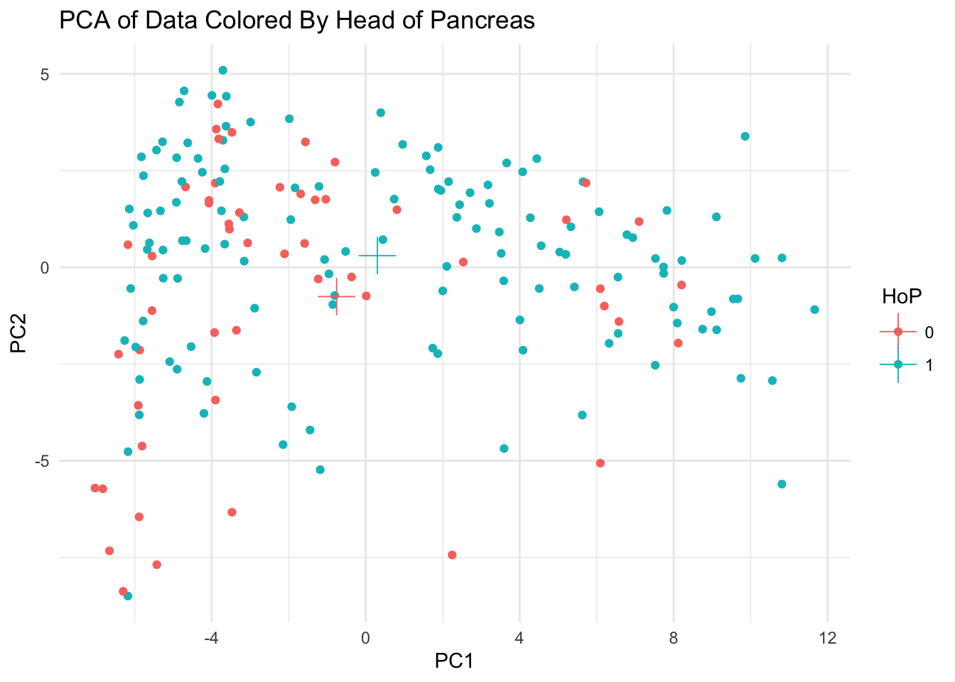
It became instantly obvious to me that MANOVA and all of the hypothesis tests for its assumptions break down with high dimensional data. I’m not sure why this is. Rather than hand picking or randomly picking a subset of variables, I perform PCA on the data and work with principal components instead.
1a. Assessing MANOVA Assumptions
group <- as.character(data_pca_df$HoP)
DVs <- data_pca_df %>% select(PC1, PC2, PC3)

# Test multivariate normality for each group (null:
# assumption met)
sapply(split(DVs, group), mshapiro_test)
## 0 1
## statistic 0.9147001 0.9350529
## p.value 0.001200223 9.521684e-06# If any p<.05, stop (assumption violated). If not,
# test homogeneity of covariance matrices
# Box's M test (null: assumption met)
# box_m(DVs, group)Welp, it appears I violate some of the assumptions of the MANOVA, but that’s no surprise. The samples are not likely to be fully random. PCA1, PC2, and PC3 are neither univariately normal nor multivariately normal. There is not a strong linear relationship between PC1, PC2, PC3 There are several groups of outliers for the variables.
Box’s test was not performed because the data did not meet the multivariate normality assumption.
1b. MANOVA: Head of Pancreas and Principal Components
man <- manova(cbind(PC1, PC2, PC3) ~ HoP, data = data_pca_df)
summary(man, tol = 0)
## Df Pillai approx F num Df den Df Pr(>F)
## HoP 1 0.10262 6.7852 3 178 0.000234 ***
## Residuals 180
## ---
## Signif. codes: 0 '***' 0.001 '**' 0.01 '*' 0.05 '.' 0.1 ' ' 1summary.aov(man)## Response PC1 :
## Df Sum Sq Mean Sq F value Pr(>F)
## HoP 1 209.8 209.843 8.114 0.004904 **
## Residuals 180 4655.1 25.862
## ---
## Signif. codes: 0 '***' 0.001 '**' 0.01 '*' 0.05 '.' 0.1 ' ' 1
##
## Response PC2 :
## Df Sum Sq Mean Sq F value Pr(>F)
## HoP 1 41.66 41.659 5.5778 0.01926 *
## Residuals 180 1344.37 7.469
## ---
## Signif. codes: 0 '***' 0.001 '**' 0.01 '*' 0.05 '.' 0.1 ' ' 1
##
## Response PC3 :
## Df Sum Sq Mean Sq F value Pr(>F)
## HoP 1 24.24 24.2394 5.4584 0.02058 *
## Residuals 180 799.34 4.4408
## ---
## Signif. codes: 0 '***' 0.001 '**' 0.01 '*' 0.05 '.' 0.1 ' ' 1pairwise.t.test((data_pca_df$PC1), data_pca_df$HoP,
p.adj = "none")##
## Pairwise comparisons using t tests with pooled SD
##
## data: (data_pca_df$PC1) and data_pca_df$HoP
##
## 0
## 1 0.0049
##
## P value adjustment method: nonepairwise.t.test((data_pca_df$PC2), data_pca_df$HoP,
p.adj = "none")##
## Pairwise comparisons using t tests with pooled SD
##
## data: (data_pca_df$PC2) and data_pca_df$HoP
##
## 0
## 1 0.019
##
## P value adjustment method: nonepairwise.t.test((data_pca_df$PC3), data_pca_df$HoP,
p.adj = "none")##
## Pairwise comparisons using t tests with pooled SD
##
## data: (data_pca_df$PC3) and data_pca_df$HoP
##
## 0
## 1 0.021
##
## P value adjustment method: nonebonf_p <- 0.05/7
bonf_p## [1] 0.007142857prob_typeI <- 1 - (0.95^7)
prob_typeI## [1] 0.3016627Significant differences were found between head of pancreas samples and non-head of pancreas samples. After performing 7 hypothesis tests, the probablility of a Type I error was 0.3016627. The bonferroni-corrected p-value is 0.007142857. While all hypothesis tests returned p-values less than 0.05. Only the MANOVA, PC1 ANOVA, and the PC1 pairwise t-test returned p-values less than the bonf_p. This means that only head of pancreas and non-head of pancreas only significantly different for principal component 1.
2a. Randomization Tests: Mean Difference in PC Values in HoP = 1 vs HoP = 0
# set the seed
set.seed(1)
# randomization_test takes a data.frame, a column
# name ('string'), and an optional iters argument
# it returns a histogram of bootstrapped mean
# distances.
randomization_test <- function(data, column, iters = 5000) {
rand_dist <- c()
new <- data %>% select(column, HoP)
for (i in 1:iters) {
temp <- new[sample(1:nrow(new), size = 10,
replace = T), ] %>% group_by(HoP) %>% summarize_if(is.numeric,
mean)
if (nrow(temp) == 1) {
rand_dist[i] <- temp %>% pull(column)
}
if (nrow(temp) == 2) {
rand_dist[i] <- temp %>% summarize_if(is.numeric,
diff) %>% pull(column)
}
}
# get the lower and upper bounds of all the
# mean_dists for that gene
lb <- quantile(rand_dist, 0.025)
ub <- quantile(rand_dist, 0.975)
data.frame(means = rand_dist) %>% ggplot(aes(x = means)) +
geom_histogram(alpha = 0.75, fill = "gray") +
theme_minimal() + geom_vline(xintercept = mean(rand_dist),
color = "red") + geom_vline(xintercept = lb,
color = "green") + geom_vline(xintercept = ub,
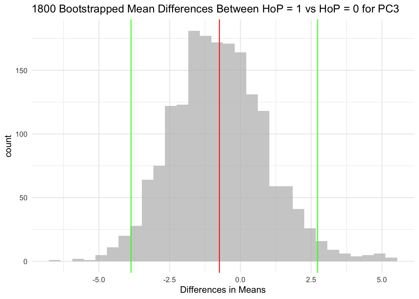
color = "green") + ggtitle(paste(i, "Bootstrapped Mean Differences Between HoP = 1 vs HoP = 0 for",
column)) + xlab("Differences in Means")
}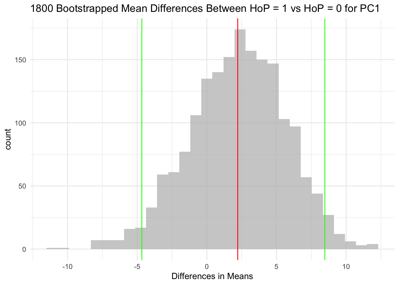

The null hypothesis for each of the three hypothesis tests is that the HoP = 1 group and HoP = 0 group do not differ in their means.
The alternative hypothesis for each of the three hypothesis tests is that the HoP = 1 group and HoP = 0 group do differ in their means.
For context, the red line in each histogram is the mean, and the green lines are the 95 CI. It’s pretty clear to me that in each of the three plots, the 95 CI encompasses 0.
The mean distributions between Head of pancreas (HoP = 1) and non-Head of pancreas (HoP = 0) samples was not significantly different for PC1, PC2, or PC3. This is because for each variable, the 95 CIs of mean differences encompass 0. I cannot reject the null hypothesis for any of these variables.
3a. LM: Predicting Survival Time from Principal Components
# create mean centered principal component
# variables; rename OS.time to `y`
data_pca_df <- data_pca_df %>% mutate(PC1_c = PC1 -
    mean(PC1), PC2_c = PC2 - mean(PC2)) %>% mutate(y = data$OS.time)


fit <- lm(y ~ PC1_c * PC2_c, data = data_pca_df)

# check normality
qqnorm(fit$residuals, main = "QQ-plot of Model Residuals")
qqline(fit$residuals, col = "red")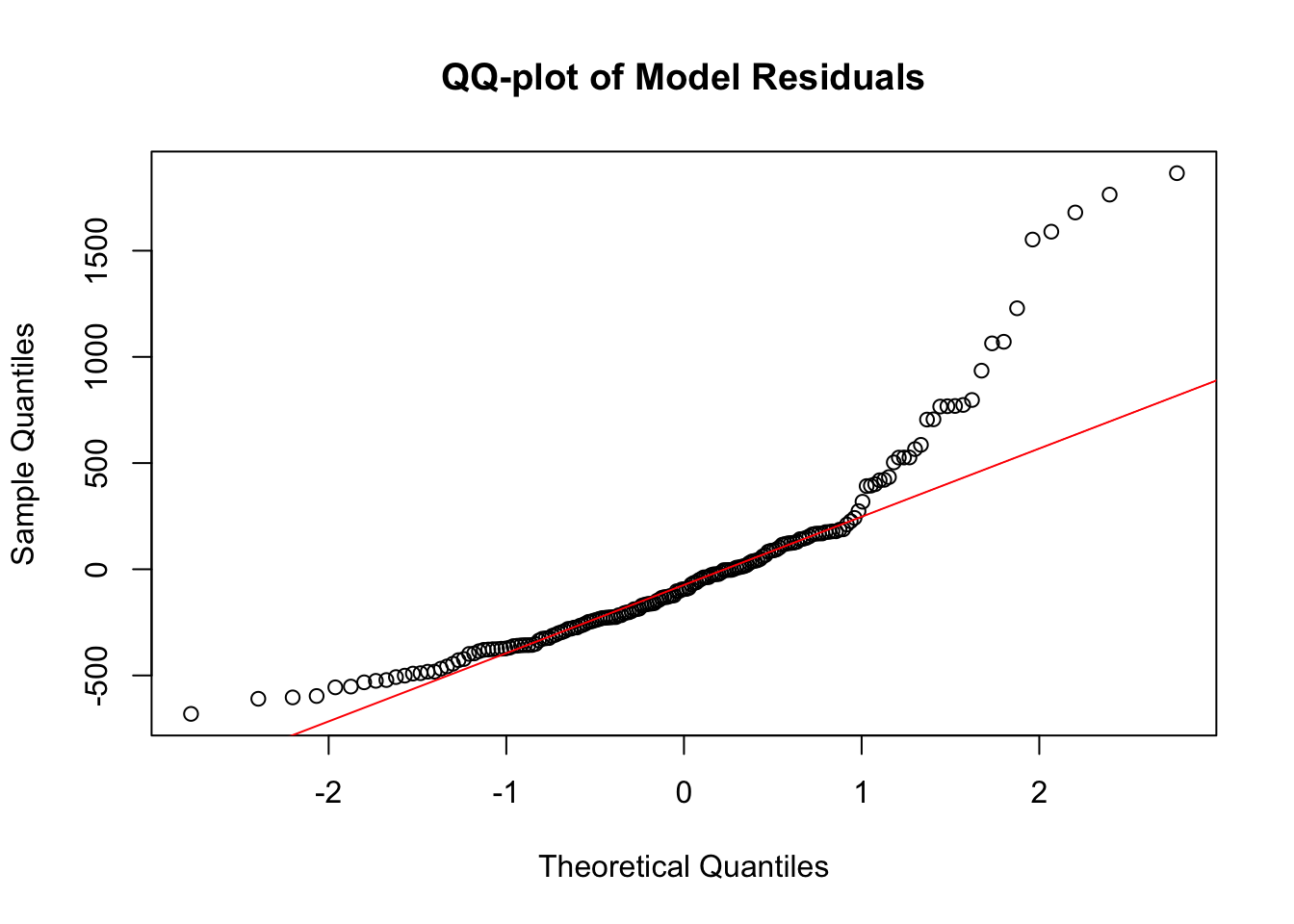
# check for uniform variance; check linearity
res <- data.frame(fitted.values = fit$fitted.values,
    residuals = fit$residuals)
res %>% ggplot(aes(fitted.values, residuals)) + geom_smooth(color = "black",
    se = T) + geom_point() + geom_hline(aes(yintercept = 0),
    color = "red") + theme_minimal() + ggtitle("Plotting Residuals by Fitted Values")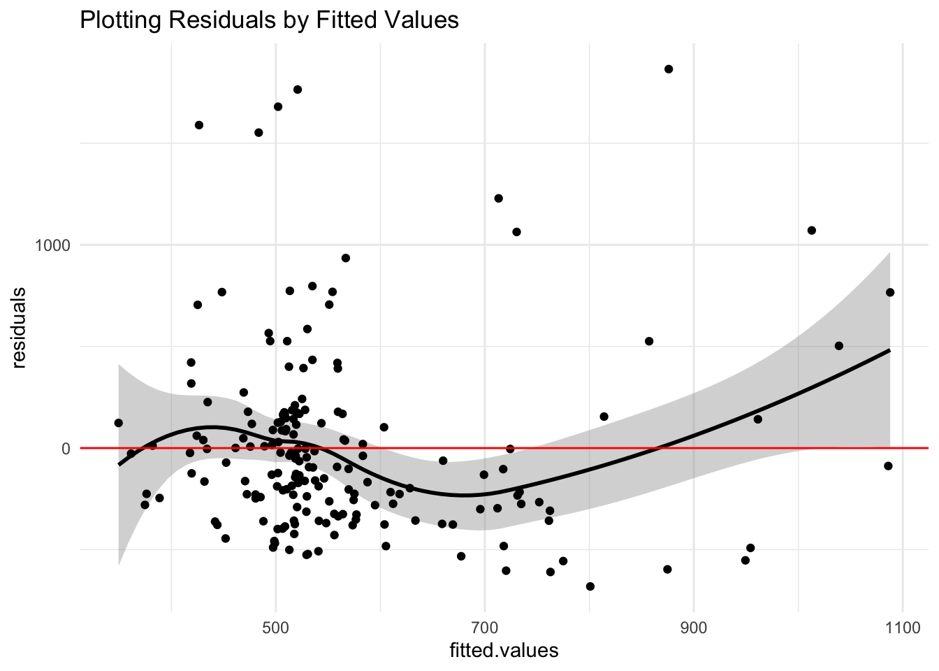
# hypothesis test for uniform variance
bptest(fit)
##
## studentized Breusch-Pagan test
##
## data: fit
## BP = 4.4287, df = 3, p-value = 0.2187# model summary
summary(fit)##
## Call:
## lm(formula = y ~ PC1_c * PC2_c, data = data_pca_df)
##
## Residuals:
## Min 1Q Median 3Q Max
## -680.91 -290.30 -93.65 143.17 1865.01
##
## Coefficients:
## Estimate Std. Error t value Pr(>|t|)
## (Intercept) 564.670 34.065 16.576 <2e-16 ***
## PC1_c -6.185 6.845 -0.904 0.3674
## PC2_c -31.236 13.778 -2.267 0.0246 *
## PC1_c:PC2_c 4.184 2.716 1.540 0.1253
## ---
## Signif. codes: 0 '***' 0.001 '**' 0.01 '*' 0.05 '.' 0.1 ' ' 1
##
## Residual standard error: 458.3 on 177 degrees of freedom
## (1 observation deleted due to missingness)
## Multiple R-squared: 0.07875, Adjusted R-squared: 0.06313
## F-statistic: 5.043 on 3 and 177 DF, p-value: 0.002236# robust SEs model summary
coeftest(fit, vcov = vcovHC(fit))##
## t test of coefficients:
##
## Estimate Std. Error t value Pr(>|t|)
## (Intercept) 564.6699 34.5618 16.3380 < 2e-16 ***
## PC1_c -6.1855 6.0165 -1.0281 0.30531
## PC2_c -31.2358 18.7447 -1.6664 0.09741 .
## PC1_c:PC2_c 4.1836 2.9188 1.4333 0.15353
## ---
## Signif. codes: 0 '***' 0.001 '**' 0.01 '*' 0.05 '.' 0.1 ' ' 1# interaction plot for PC1_c, PC2_c
interact_plot(fit, pred = PC1_c, modx = PC2_c, data = data_pca_df)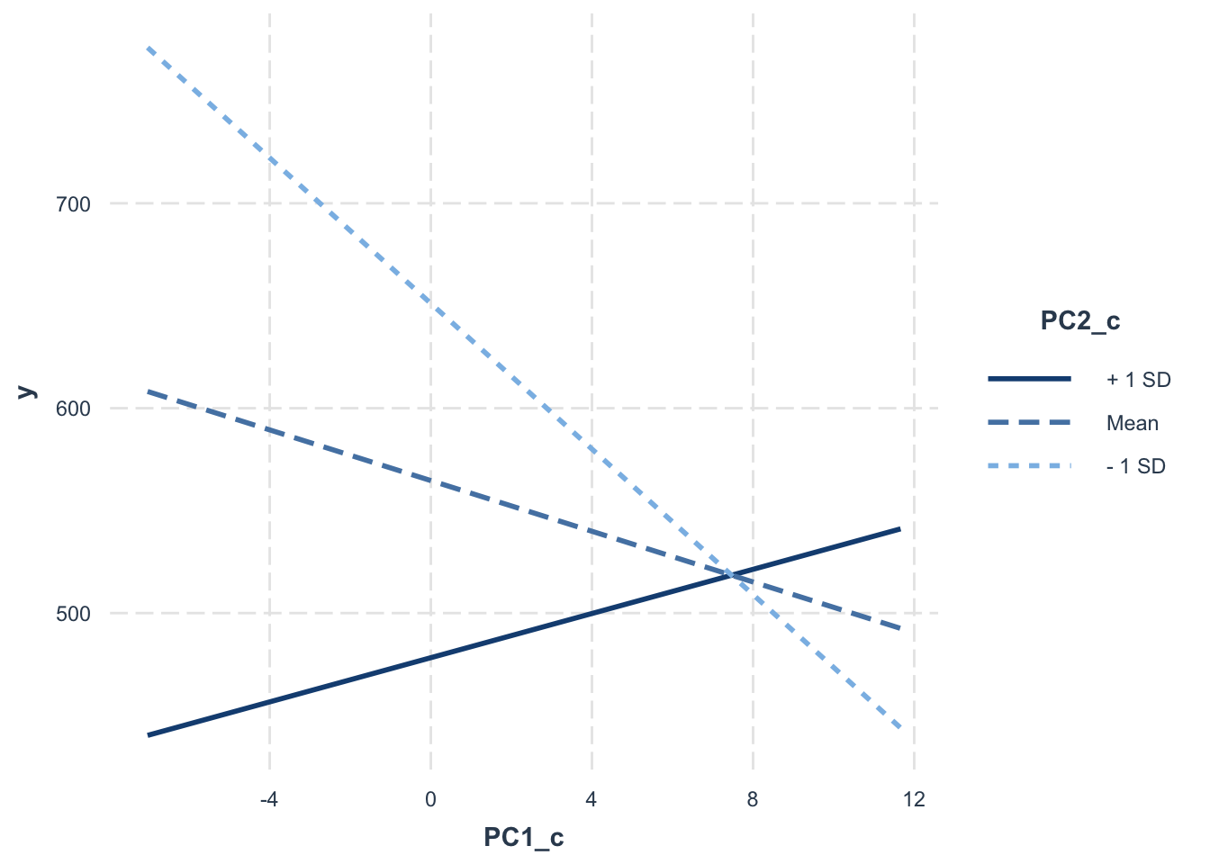
OS.time =564.67 - 6.185(PC1_c) - 31.236(PC2_c) + 4.184(PC1_c * PC2_c)
It’s clear from the QQ plot that my data is not normal at all. That said, the BP Test and even distribution of residuals around 0 prove show that the data is homoskedastic and exhibits a linear trend.
For samples of average PC1 and PC2, the predicted overall survival time is 564.67 days. PC1_c has a coefficient of -6.185. This means that for every one-unit increase in PC1_c, OS.time decreases by 6.185, on average. (not significant) PC2_c has a coefficient of -31.236. This means that for every one-unit increase in PC2_c, OS.time decreases by 31.236, on average. (significant) The coefficent for PC1_c:PC2_c is 4.184. This shows that as PC2_c increases, the effect of PC1_c on OS.time becomes more positive. (not significant)
This model has an adjusted R-squared of 0.06313; this means that my model explains 6.313% of the variation in OS.time
The Robust SE LM returned no significant coefficients save for the intercept. This means that because Robust SEs were used, PC2_c is no longer a significant predictor of Head of Pancreas.
4a. Bootstrapped SE LM
set.seed(1)

samp_distn <- replicate(5000, {
    boot_dat <- sample_frac(data_pca_df, replace = T)

    fit <- lm(y ~ PC1_c * PC2_c, data = boot_dat)
    coef(fit)
})

samp_distn %>% t %>% as.data.frame %>% summarize_all(sd)
## (Intercept) PC1_c PC2_c PC1_c:PC2_c
## 1 33.60516 6.041935 18.34254 2.882069samp_distn %>% t %>% as.data.frame %>% pivot_longer(everything()) %>%
group_by(name) %>% summarize(lower = quantile(value,
0.025), upper = quantile(value, 0.975))## # A tibble: 4 x 3
## name lower upper
## <chr> <dbl> <dbl>
## 1 (Intercept) 500. 631.
## 2 PC1_c -17.2 6.12
## 3 PC1_c:PC2_c -1.79 9.72
## 4 PC2_c -66.0 5.87The intercept’s 95 CI does not cross 0 and is significant. All other 95 CIs include 0 and indicate that the other variables are not significant predictors. This yielded the same results as the Robust SEs LM.
5a. Define class_diag and conf_matrix functions with optional decision threshold parameters
class_diag <- function(probs, truth, thresh = 0.5) {
    tab <- table(factor(probs > thresh, levels = c("FALSE",
        "TRUE")), truth)
    acc = sum(diag(tab))/sum(tab)
    sens = tab[2, 2]/colSums(tab)[2]
    spec = tab[1, 1]/colSums(tab)[1]
    ppv = tab[2, 2]/rowSums(tab)[2]
    f1 = 2 * (sens * ppv)/(sens + ppv)

    if (is.numeric(truth) == FALSE & is.logical(truth) ==
        FALSE) {
        truth <- as.numeric(truth) - 1
    }

    # CALCULATE EXACT AUC
    ord <- order(probs, decreasing = TRUE)
    probs <- probs[ord]
    truth <- truth[ord]

    TPR = cumsum(truth)/max(1, sum(truth))
    FPR = cumsum(!truth)/max(1, sum(!truth))

    dup <- c(probs[-1] >= probs[-length(probs)], FALSE)
    TPR <- c(0, TPR[!dup], 1)
    FPR <- c(0, FPR[!dup], 1)

    n <- length(TPR)
    auc <- sum(((TPR[-1] + TPR[-n])/2) * (FPR[-1] -
        FPR[-n]))

    data.frame(acc, sens, spec, ppv, f1, auc)
}
# prints a confusion matrix to the screen
conf_matrix <- function(probs, truth, thresh = 0.5) {
    table(factor(probs > thresh, levels = c("FALSE",
        "TRUE")), truth)
}

# find optimal thresh optimizes the decision
# threshold to yield the maximum f1 score
find_optimal_thresh <- function(fit, data_genes, probs,
    plot = FALSE) {
    data_genes$probs <- probs
    # initialize f_df variable
    f_df <- NULL
    # for i in 1000 iterations, get the f1-score for
    # every possible cutoff between 0 and 1,
    # incrementing 0.001 each iteration
    for (i in 1:1000) {
        f_df <- rbind(f_df, data.frame(cutoff = i/1000,
            f1 = class_diag(data_genes$probs, data_genes$Head_of_pancreas,
                i/1000)$f1))
    }

    # get decision threshold that yielded the highest
    # F1-score
    thresh <- (f_df %>% arrange(desc(f1)))[1, ] %>%
        pull(cutoff)
    if (plot == TRUE) {
        print(ggplot(f_df, aes(cutoff, f1)) + geom_line() +
            geom_vline(aes(xintercept = thresh)) +
            xlab("Decision Threshold") + ylab("F1-score") +
            theme_minimal() + ggtitle("Identifying the Optimal Decision Threshold"))
    }


    return(thresh)
}

# generate density plot separated by
# head_of_pancreas group
logit_density <- function(fit, Head_of_pancreas) {
    # plot frequency plot of logit for both classes
    print(data.frame(predict = predict(fit, type = "link"),
        Head_of_pancreas = Head_of_pancreas) %>% ggplot(aes(predict)) +
        geom_density(aes(fill = Head_of_pancreas),
            alpha = 0.5) + theme_minimal() + geom_vline(aes(xintercept = 0)) +
        xlab("logit"))
}
5b. Logistic Regression Predicting Head of Pancreas from Three Randomly Picked Genes
set.seed(5)
data_genes <- data %>% select(Head_of_pancreas, contains("ENSG"))
data_genes <- data_genes %>% select(sample(2:ncol(data_genes),
    3), Head_of_pancreas)
fit <- glm(Head_of_pancreas ~ ., family = "binomial",
    data = data_genes, control = list(maxit = 75))

# get class probabilities
data_genes$probs <- predict(fit, type = "response")
summary(fit)
##
## Call:
## glm(formula = Head_of_pancreas ~ ., family = "binomial", data = data_genes,
## control = list(maxit = 75))
##
## Deviance Residuals:
## Min 1Q Median 3Q Max
## -1.9616 -1.3477 0.6723 0.9301 1.0202
##
## Coefficients:
## Estimate Std. Error z value Pr(>|z|)
## (Intercept) 0.39463 0.24572 1.606 0.108
## ENSG00000169347.15 0.07724 0.13142 0.588 0.557
## ENSG00000179751.6 0.17209 0.28277 0.609 0.543
## ENSG00000142615.7 -0.10031 0.25401 -0.395 0.693
##
## (Dispersion parameter for binomial family taken to be 1)
##
## Null deviance: 217.77 on 181 degrees of freedom
## Residual deviance: 208.19 on 178 degrees of freedom
## AIC: 216.19
##
## Number of Fisher Scoring iterations: 4exp(coef(fit))## (Intercept) ENSG00000169347.15 ENSG00000179751.6 ENSG00000142615.7
## 1.4838370 1.0803008 1.1877791 0.9045531thresh <- find_optimal_thresh(fit, data_genes, data_genes$probs,
TRUE)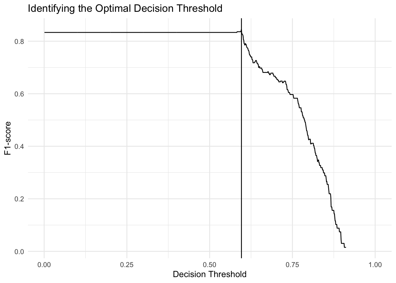
# get relevant metrics on fit
class_diag(data_genes$probs, data$Head_of_pancreas,
    thresh)
## acc sens spec ppv f1 auc
## 1 0.7417582 0.9923077 0.1153846 0.7371429 0.8459016 0.6445266# generate confusion matrix of fit
conf_matrix(data_genes$probs, data$Head_of_pancreas,
thresh)## truth
## 0 1
## FALSE 6 1
## TRUE 46 129logit_density(fit, data_genes$Head_of_pancreas)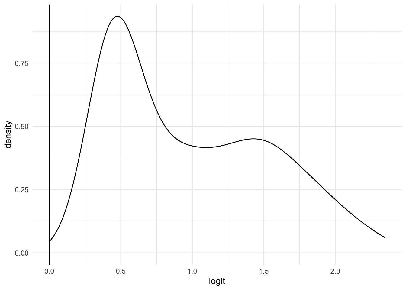
ggplot(data_genes) + geom_roc(aes(d = as.numeric(Head_of_pancreas),
    m = probs), n.cuts = 0)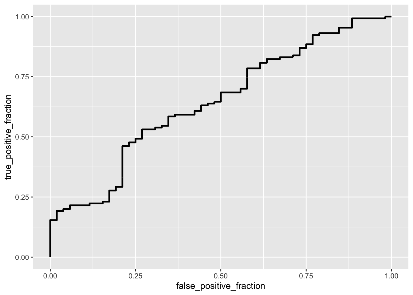
For this one I picked three random genes with which to work.
log(odds of class 1) = 0.07724(ENSG00000169347.15) - 0.17209(ENSG00000175535.6) + 0.10031(ENSG00000164266.9) + 0.39463
Log odds are hard to intrepret, so I exponentiate all of the coefficients.
Controlling for ENSG00000175535.6 and ENSG00000164266.9, each one unit increase in ENSG00000169347.15 increases the odds of being class 1 by a factor of 1.0803008 (not significant)
Controlling for ENSG00000169347.15 and ENSG00000164266.9, each one unit increase in ENSG00000175535.6 increases the odds of being class 1 by a factor of 1.1877791 (not significant)
Controlling for ENSG00000169347.15 ENSG00000175535.6, each one unit increase in ENSG00000164266.9 increases the odds of being class 1 by a factor of 0.9045531 (not significant)
Immediately, it’s clear that this model sacrifices specificity (0.1153846) for sensitivity (0.9923077). The model’s accuracy is 0.7417582 and its precision is 0.7371429 The F1-score is surprisingly high (0.8459016), which is never bad. The AUC is a lousy 0.6445266.
The ROC curve has a very low AUC (0.6445266). This means that the model cannot achieve a high TPR without incurring a high FPR.
6a. Predicting Head of Pancreas from All Genes
# pull out genes, head of pancreas
data_genes <- data %>% select(contains("ENSG"), Head_of_pancreas)
# fit logistic model to all genes; predict log odds
# of Head_of_pancreas; maxit = 75 prevents model
# from failing with large numbers of variables
fit <- glm(Head_of_pancreas ~ ., family = "binomial",
    data = data_genes, control = list(maxit = 75))
# get class probabilities
data_genes$probs <- predict(fit, type = "response")
summary(fit)
##
## Call:
## glm(formula = Head_of_pancreas ~ ., family = "binomial", data = data_genes,
## control = list(maxit = 75))
##
## Deviance Residuals:
## Min 1Q Median 3Q Max
## -2.85033 -0.05722 0.11068 0.48014 1.84377
##
## Coefficients:
## Estimate Std. Error z value Pr(>|z|)
## (Intercept) -1.563394 2.983896 -0.524 0.60032
## ENSG00000164266.9 0.102611 0.277310 0.370 0.71136
## ENSG00000169347.15 0.344227 0.418384 0.823 0.41065
## ENSG00000175535.6 -0.667590 1.139099 -0.586 0.55783
## ENSG00000215704.8 1.631599 1.326965 1.230 0.21886
## ENSG00000211892.3 -0.027101 0.226791 -0.119 0.90488
## ENSG00000243480.6 -1.252604 0.643884 -1.945 0.05173 .
## ENSG00000096006.10 -0.307265 0.267720 -1.148 0.25109
## ENSG00000118271.8 0.671077 0.707698 0.948 0.34300
## ENSG00000219073.6 -0.824490 1.552025 -0.531 0.59526
## ENSG00000066405.11 -0.555978 0.335348 -1.658 0.09733 .
## ENSG00000122711.7 -0.026514 0.288477 -0.092 0.92677
## ENSG00000108849.6 0.145380 0.196099 0.741 0.45848
## ENSG00000170890.12 -2.180794 1.493387 -1.460 0.14421
## ENSG00000256618.2 0.034362 0.158207 0.217 0.82805
## ENSG00000175084.10 0.186929 0.189869 0.985 0.32486
## ENSG00000254647.5 0.476140 0.325111 1.465 0.14304
## ENSG00000134193.13 0.512320 0.248319 2.063 0.03910 *
## ENSG00000275896.3 -0.096492 0.460265 -0.210 0.83395
## ENSG00000167653.4 0.089175 0.156002 0.572 0.56757
## [ reached getOption("max.print") -- omitted 42 rows ]
## ---
## Signif. codes: 0 '***' 0.001 '**' 0.01 '*' 0.05 '.' 0.1 ' ' 1
##
## (Dispersion parameter for binomial family taken to be 1)
##
## Null deviance: 217.77 on 181 degrees of freedom
## Residual deviance: 104.19 on 120 degrees of freedom
## AIC: 228.19
##
## Number of Fisher Scoring iterations: 8thresh <- find_optimal_thresh(fit, data_genes, data_genes$probs,
TRUE)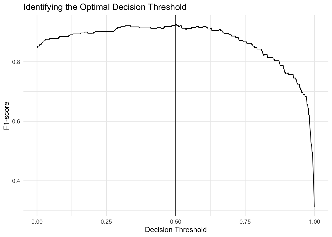
# get relevant metrics on fit
class_diag(data_genes$probs, data$Head_of_pancreas,
    thresh)
## acc sens spec ppv f1 auc
## 1 0.8901099 0.9538462 0.7307692 0.8985507 0.9253731 0.9322485# generate confusion matrix of fit
conf_matrix(data_genes$probs, data$Head_of_pancreas,
thresh)## truth
## 0 1
## FALSE 38 6
## TRUE 14 124# generate ROC curve for fit
ggplot(data_genes) + geom_roc(aes(d = as.numeric(Head_of_pancreas),
m = probs), n.cuts = 0)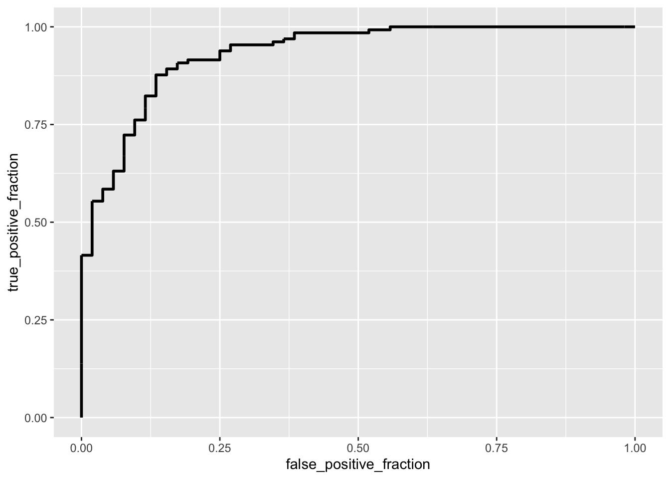
logit_density(fit, data_genes$Head_of_pancreas)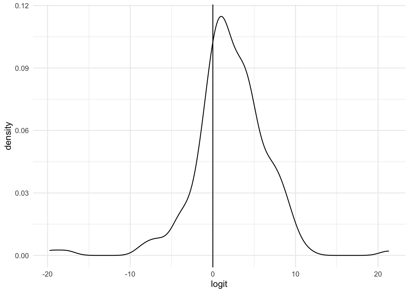
There are too many coefficients to count, but I’ll provide a template for their interpretation: variable has a coefficient of coeff. This means that for every one-unit increase in variable, log odds of head of pancreas (increases/decreases) by coeff. (if Pr(>|z|) < 0.05: significant; else: not significant)
The model classifies 38 of the 52 false values as false. It classifies 124 of the 130 positive values as positive.
The model performs very well. It is somewhat more sensitive (0.95) than it is specific (0.73); it gets a high accuracy (0.89); it has a precision of 0.899; it has a great f1 (0.925). The AUC is a great 0.932.
The optimal decision threshold for this model is at probability = 0.498; anything above is classified a Head of Pancreas sample. Anything below is non-head of pancreas.
The ROC curve has a very large AUC (0.932). This means that the model can achieve a very high TPR while maintaining a relatively low FPR.
6b. 10 fold CV with all variables
data_genes <- data %>% select(contains("ENSG"), Head_of_pancreas)
k = 10
temp <- data_genes[sample(nrow(data_genes)), ]
folds <- cut(seq(1:nrow(data_genes)), breaks = k, labels = F)
diags <- NULL
for (i in 1:k) {
    train <- temp[folds != i, ]  #create training set (all but fold i)
    test <- temp[folds == i, ]  #create test set (just fold i)
    truth <- test$Head_of_pancreas  #save truth labels from fold i
    fit <- glm(Head_of_pancreas ~ ., family = "binomial",
        data = train, control = list(maxit = 75))
    probs <- predict(fit, newdata = test, type = "response")
    thresh <- find_optimal_thresh(fit, train, predict(fit,
        type = "response"))
    diags <- rbind(diags, class_diag(probs, truth,
        thresh))
}
summarize_all(diags, mean)
## acc sens spec ppv f1 auc
## 1 0.6312865 0.7257792 0.3980952 0.7486476 0.731227 0.5923399The 10-fold CV has exposed the degree to which the previous model had overfitted to the dataset. Even with optimal decision cutoffs, the AUC was only 0.632. Accuracy, sensitivity, specificity, precision, and f1 are 0.7186647, 0.442619, 0.7710556, and 0.7384776, respectively.
6c. LASSO
set.seed(1234)
data_genes <- data %>% select(contains("ENSG"), Head_of_pancreas)
y <- as.matrix(data_genes$Head_of_pancreas)
preds <- model.matrix(Head_of_pancreas ~ ., data = data_genes)[,
    -1] %>% scale
cv <- cv.glmnet(preds, y, family = "binomial")
{
    plot(cv$glmnet.fit, "lambda", label = TRUE)
    abline(v = log(cv$lambda.1se))
}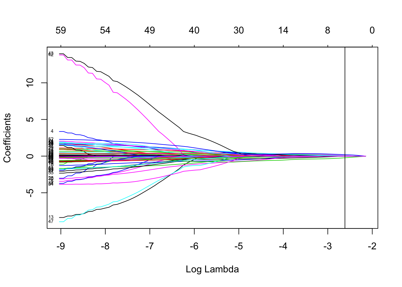
lasso_fit <- glmnet(preds, y, family = "binomial",
    lambda = cv$lambda.1se)
# probs <- predict(lasso_fit, preds,
# type='response')
# class_diag(probs,data_genes$Head_of_pancreas,0.5)
# conf_matrix(probs,data_genes$Head_of_pancreas)
x <- coef(lasso_fit)
rownames(x)[x[, 1] > 0]
## [1] "(Intercept)" "ENSG00000108849.6" "ENSG00000175084.10"
## [4] "ENSG00000188257.9" "ENSG00000172016.14"LASSO selected four genes as effective predictors:“ENSG00000108849.6” “ENSG00000175084.10” “ENSG00000188257.9” “ENSG00000172016.14”. Using these variables to train a model will make it much more generalizable.
6d. 10-fold CV on LASSO-honed Logistic Model
data_genes <- data %>% select(ENSG00000108849.6, ENSG00000175084.10,
    ENSG00000188257.9, ENSG00000172016.14, Head_of_pancreas)
k = 10
temp <- data_genes[sample(nrow(data_genes)), ]
folds <- cut(seq(1:nrow(data_genes)), breaks = k, labels = F)
diags <- NULL
for (i in 1:k) {
    train <- temp[folds != i, ]  #create training set (all but fold i)
    test <- temp[folds == i, ]  #create test set (just fold i)
    truth <- test$Head_of_pancreas  #save truth labels from fold i
    fit <- glm(Head_of_pancreas ~ ., family = "binomial",
        data = train)
    probs <- predict(fit, newdata = test, type = "response")
    thresh <- find_optimal_thresh(fit, train, predict(fit,
        type = "response"))
    diags <- rbind(diags, class_diag(probs, truth,
        thresh))
}
summarize_all(diags, mean)
## acc sens spec ppv f1 auc
## 1 0.7312865 0.9149567 0.2194444 0.745767 0.8189543 0.6573088I suppose this is the best I can do given the tools we’ve learned in this course. The AUC is terrible (0.680). While sensitivity is great (0.93), specificity is non-existent (0.1). This tells me that the decision threshold chosen for my model is basically near 0, and it is classifying everything as Head of pancreas. Accuracy is bad, but not atrocious (0.69). Precision and f1 score are 0.72 and 0.81, respectively.
Although this model gets lower scores than some of its predecessors, it is much more generalizable than those previous models and will thus perform better than them on new data.
## R version 3.6.0 (2019-04-26)
## Platform: x86_64-apple-darwin15.6.0 (64-bit)
## Running under: macOS  10.15.6
##
## Matrix products: default
## BLAS:   /Library/Frameworks/R.framework/Versions/3.6/Resources/lib/libRblas.0.dylib
## LAPACK: /Library/Frameworks/R.framework/Versions/3.6/Resources/lib/libRlapack.dylib
##
## locale:
## [1] en_US.UTF-8/en_US.UTF-8/en_US.UTF-8/C/en_US.UTF-8/en_US.UTF-8
##
## attached base packages:
## [1] grid      stats     graphics  grDevices utils     datasets  methods
## [8] base
##
## other attached packages:
##  [1] rstatix_0.5.0        interactions_1.1.3   factoextra_1.0.7
##  [4] circlize_0.4.9       ComplexHeatmap_2.0.0 reshape2_1.4.4
##  [7] prettyR_2.2-3        glmnet_4.0-2         Matrix_1.2-18
## [10] plotROC_2.2.1        lmtest_0.9-38        zoo_1.8-8
## [13] sandwich_3.0-0       forcats_0.5.0        stringr_1.4.0
## [16] dplyr_1.0.0          purrr_0.3.4          tidyr_1.1.0
## [19] tibble_3.0.1         ggplot2_3.3.1        tidyverse_1.3.0
## [22] readr_1.3.1
##
## loaded via a namespace (and not attached):
##  [1] nlme_3.1-148        fs_1.4.1            lubridate_1.7.9
##  [4] RColorBrewer_1.1-2  httr_1.4.1          tools_3.6.0
##  [7] backports_1.1.7     utf8_1.1.4          R6_2.4.1
## [10] mgcv_1.8-31         DBI_1.1.0           colorspace_1.4-1
## [13] GetoptLong_0.1.8    withr_2.2.0         tidyselect_1.1.0
## [16] curl_4.3            compiler_3.6.0      cli_2.0.2
## [19] rvest_0.3.5         formatR_1.7         xml2_1.3.2
## [22] labeling_0.3        bookdown_0.19       scales_1.1.1
## [25] digest_0.6.25       foreign_0.8-72      rmarkdown_2.2
## [28] rio_0.5.16          pkgconfig_2.0.3     htmltools_0.4.0
## [31] dbplyr_1.4.4        rlang_0.4.6         GlobalOptions_0.1.1
## [34] readxl_1.3.1        rstudioapi_0.11     farver_2.0.3
## [37] shape_1.4.4         generics_0.0.2      jsonlite_1.6.1
## [40] zip_2.0.4           car_3.0-8           magrittr_1.5
## [43] Rcpp_1.0.5          munsell_0.5.0       fansi_0.4.1
## [46] abind_1.4-5         lifecycle_0.2.0     stringi_1.4.6
## [49] yaml_2.2.1          carData_3.0-4       plyr_1.8.6
## [52] blob_1.2.1          parallel_3.6.0      ggrepel_0.8.2
## [55] crayon_1.3.4        lattice_0.20-41     haven_2.3.1
## [58] splines_3.6.0       jtools_2.1.0        pander_0.6.3
## [61] hms_0.5.3           knitr_1.28          pillar_1.4.4
## [64] rjson_0.2.20        codetools_0.2-16    reprex_0.3.0
## [67] glue_1.4.1          evaluate_0.14       blogdown_0.19
## [70] data.table_1.12.8   modelr_0.1.8        png_0.1-7
## [73] vctrs_0.3.1         foreach_1.5.0       cellranger_1.1.0
## [76] gtable_0.3.0        clue_0.3-57         assertthat_0.2.1
## [79] openxlsx_4.1.5      xfun_0.14           broom_0.5.6
## [82] survival_3.1-12     iterators_1.0.12    cluster_2.1.0
## [85] ellipsis_0.3.1
## [1] "2020-12-08 23:18:44 CST"## sysname
## "Darwin"
## release
## "19.6.0"
## version
## "Darwin Kernel Version 19.6.0: Thu Jun 18 20:49:00 PDT 2020; root:xnu-6153.141.1~1/RELEASE_X86_64"
## nodename
## "Extension.local"
## machine
## "x86_64"
## login
## "root"
## user
## "ryanbailey"
## effective_user
## "ryanbailey"Ryan Bailey
Medical Student, Bioinformatician, and Photographer in San Antonio, Texas.
My interests include unsupervised learning, oncology, software engineering. matter.