The Beauty of Reticulate
 Photo by Romina Farías on Unsplash
Python and R are integral to data science, period. There is no way around using them. Each language is great in its own right, but together, they’re unstoppable. In the below notebook, I am training a scikit-learn Support Vector Machine (SVM) classifier on Diabetic Retinopathy Debrecen Dataset. If you’re unfamiliar with SVMs, I highly recommend this article by Rohith Gandhi from the Towards Data Science blog on Medium. After we build the classifier, I do some hyperparameter tuning until I reach a reasonable accuracy.
All this stuff can be done in Python easily. But I want to use ggplot to visualize the dataset. Reticulate lets R and Python communicate with each others’ environment. After I finish the classifier, I reduced the dimensionality of the dataset via UMAP. At the very bottom of the notebook, I show how the SVM’s predict functionality is preserved from Python to R.
Load in the Reticulate library
library(reticulate)Check the Python configuration to make sure the paths and versions look good
py_config()## python: /Users/ryanbailey/Library/r-miniconda/envs/r-reticulate/bin/python
## libpython: /Users/ryanbailey/Library/r-miniconda/envs/r-reticulate/lib/libpython3.6m.dylib
## pythonhome: /Users/ryanbailey/Library/r-miniconda/envs/r-reticulate:/Users/ryanbailey/Library/r-miniconda/envs/r-reticulate
## version: 3.6.11 | packaged by conda-forge | (default, Aug 5 2020, 20:19:23) [GCC Clang 10.0.1 ]
## numpy: /Users/ryanbailey/Library/r-miniconda/envs/r-reticulate/lib/python3.6/site-packages/numpy
## numpy_version: 1.19.4Importing Packages
#!/usr/bin/env python
# coding: utf-8

#You may add additional imports
import warnings
warnings.simplefilter("ignore")
import pandas as pd
import numpy as np
import sklearn as sk
import matplotlib.pyplot as plt
import time
from sklearn.model_selection import GridSearchCV as GSCV
from sklearn.model_selection import cross_val_score
##Load in the dataset (Diabetic Retinopathy Debrecen Data Set)
col_names = []
for i in range(20):
    if i == 0:
        col_names.append('quality')
    if i == 1:
        col_names.append('prescreen')
    if i >= 2 and i <= 7:
        col_names.append('ma' + str(i))
    if i >= 8 and i <= 15:
        col_names.append('exudate' + str(i))
    if i == 16:
        col_names.append('euDist')
    if i == 17:
        col_names.append('diameter')
    if i == 18:
        col_names.append('amfm_class')
    if i == 19:
        col_names.append('label')

data = pd.read_csv("messidor_features.txt", names = col_names)
print(data.shape)
## (1151, 20)data.head(10)## quality prescreen ma2 ma3 ... euDist diameter amfm_class label
## 0 1 1 22 22 ... 0.486903 0.100025 1 0
## 1 1 1 24 24 ... 0.520908 0.144414 0 0
## 2 1 1 62 60 ... 0.530904 0.128548 0 1
## 3 1 1 55 53 ... 0.483284 0.114790 0 0
## 4 1 1 44 44 ... 0.475935 0.123572 0 1
## 5 1 1 44 43 ... 0.502831 0.126741 0 1
## 6 1 0 29 29 ... 0.541743 0.139575 0 1
## 7 1 1 6 6 ... 0.576318 0.071071 1 0
## 8 1 1 22 21 ... 0.500073 0.116793 0 1
## 9 1 1 79 75 ... 0.560959 0.109134 0 1
##
## [10 rows x 20 columns]datay = data['label']
datax = data.drop('label',axis =1 )
print(datay.shape)## (1151,)print(datax.shape)## (1151, 19)datax.head()## quality prescreen ma2 ma3 ... exudate15 euDist diameter amfm_class
## 0 1 1 22 22 ... 0.003923 0.486903 0.100025 1
## 1 1 1 24 24 ... 0.003903 0.520908 0.144414 0
## 2 1 1 62 60 ... 0.007744 0.530904 0.128548 0
## 3 1 1 55 53 ... 0.001531 0.483284 0.114790 0
## 4 1 1 44 44 ... 0.000000 0.475935 0.123572 0
##
## [5 rows x 19 columns]Building a pipeline to first scale the data, then to train the model
from sklearn.preprocessing import StandardScaler as SS
from sklearn.svm import SVC
from sklearn.pipeline import Pipeline
SS = SS()
clf = SVC()
pipe = Pipeline(steps=[('scaler', SS), ('SVC', clf)])

nested_score = cross_val_score(pipe, datax, datay, cv=5)
print('Mean Nested Score:',nested_score.mean())
## Mean Nested Score: 0.7011368341803125Hyperparameter Tuning
# for the 'svm' part of the pipeline, tune the 'kernel' hyperparameter
param_grid = {'SVC__kernel': ['linear', 'rbf', 'poly', 'sigmoid']}
grid_search = GSCV(pipe, param_grid, cv=5, scoring='accuracy')
grid_search.fit(datax,datay)
## GridSearchCV(cv=5,
## estimator=Pipeline(steps=[('scaler', StandardScaler()),
## ('SVC', SVC())]),
## param_grid={'SVC__kernel': ['linear', 'rbf', 'poly', 'sigmoid']},
## scoring='accuracy')best_kernel = grid_search.best_params_.get('SVC__kernel')
print(grid_search.best_params_)## {'SVC__kernel': 'linear'}print("Accuracy:", grid_search.best_score_)## Accuracy: 0.7228646715603239Nested cross validation mean accuracy
nested_score = cross_val_score(grid_search, datax, datay, cv=5)
print('Mean Nested Score: ',nested_score.mean())
## Mean Nested Score: 0.7228646715603239Cross Validating the Hyperparameter-tuned Model
param_grid = {'SVC__kernel': ['linear', 'rbf', 'poly', 'sigmoid'],'SVC__C':list(range(50,110,10))}
grid_search = GSCV(pipe, param_grid, cv=5, scoring='accuracy')
grid_search.fit(datax,datay)
## GridSearchCV(cv=5,
## estimator=Pipeline(steps=[('scaler', StandardScaler()),
## ('SVC', SVC())]),
## param_grid={'SVC__C': [50, 60, 70, 80, 90, 100],
## 'SVC__kernel': ['linear', 'rbf', 'poly', 'sigmoid']},
## scoring='accuracy')best_kernel = grid_search.best_params_.get('SVC__kernel')
print(grid_search.best_params_)## {'SVC__C': 70, 'SVC__kernel': 'linear'}print("Accuracy:", grid_search.best_score_)## Accuracy: 0.7463052889139845nested_score = cross_val_score(grid_search, datax, datay, cv=5)
print('Mean Nested Score:',nested_score.mean())
## Mean Nested Score: 0.7454357236965933Loading in R packages
library(umap)## Warning: package 'umap' was built under R version 3.6.2library(readr)
library(tidyverse)## ── Attaching packages ──────────────────────────────────────────────────────────────── tidyverse 1.3.0 ──## ✓ ggplot2 3.3.1 ✓ dplyr 1.0.0
## ✓ tibble 3.0.1 ✓ stringr 1.4.0
## ✓ tidyr 1.1.0 ✓ forcats 0.5.0
## ✓ purrr 0.3.4## Warning: package 'ggplot2' was built under R version 3.6.2## Warning: package 'tibble' was built under R version 3.6.2## Warning: package 'tidyr' was built under R version 3.6.2## Warning: package 'purrr' was built under R version 3.6.2## Warning: package 'dplyr' was built under R version 3.6.2## ── Conflicts ─────────────────────────────────────────────────────────────────── tidyverse_conflicts() ──
## x dplyr::filter() masks stats::filter()
## x dplyr::lag() masks stats::lag()library(ggplot2)
library(ggalt)## Registered S3 methods overwritten by 'ggalt':
## method from
## grid.draw.absoluteGrob ggplot2
## grobHeight.absoluteGrob ggplot2
## grobWidth.absoluteGrob ggplot2
## grobX.absoluteGrob ggplot2
## grobY.absoluteGrob ggplot2library(ggforce)## Warning: package 'ggforce' was built under R version 3.6.2library(concaveman)## Warning: package 'concaveman' was built under R version 3.6.2Collapsing the data with UMAP
set.seed(3)
labels <- py$data %>% pull(label)
data <- py$data %>% select(-label)
data_umap = umap(data)
umap_features <- cbind(((data_umap$layout) %>% as.data.frame),labels) %>%
  mutate(label = as.factor(labels)) %>%
  select(-labels)
umap_features %>% head
## V1 V2 label
## 1 -1.5948603 2.517664 0
## 2 -1.2361083 2.352496 0
## 3 0.8065302 -2.698501 1
## 4 -0.1869378 -3.680573 0
## 5 -3.2231895 -3.336815 1
## 6 -2.6021497 -2.833544 1Plot the UMAP Data
umap_features %>%
  ggplot(aes(x = V1, y =V2, color = as.factor(labels))) +
  geom_point(size = 3) + theme_minimal() +
  geom_mark_ellipse(expand = 0,aes(fill=as.factor(labels))) +
  xlab("UMAP Feature 1") +
  ylab("UMAP Feature 2")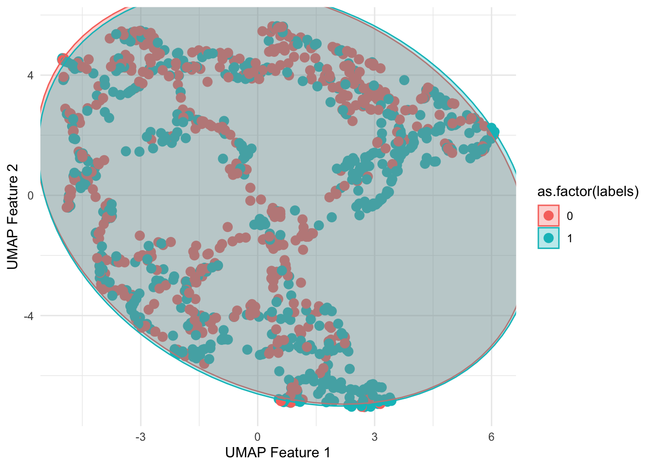
Extracting the predict method from the SVM
predict <- py$grid_search$predict
set.seed(1)
predict(data[sample(1:nrow(data),2),])
## [1] 0 1Ryan Bailey
Medical Student, Bioinformatician, and Photographer in San Antonio, Texas.
My interests include unsupervised learning, oncology, software engineering. matter.